Media Tables

Data Model of Spiral Tables makes them an ideal choice for storing and managing large-scale multimodal datasets (including images, videos, audio files, text, transformer-based embeddings and more). Tables are designed to store both data and traditional metadata (labels, annotations, complex nested data and more) in a single model.

Let’s build a table of crawled image data.

Start from Metadata

First, create a table with a composite primary key made up of page_url and key columns. Spiral Tables have primary keys that can consist of multiple columns, and are used as both sort order as well as to support updates and zero-copy appends. In this case, key represents a unique identifier for each media item on the page identified by page_url.


from spiral import Spiral
import pyarrow as pa
 
sp = Spiral()
project = sp.project("example")
 
table = project.create_table(
    "media-table",
    key_schema=pa.schema({"page_url": pa.string(), "key": pa.int64()})
)

While it’s possible to write raw data (images, audio, video, etc.) directly into Spiral Tables, it’s much more common to start from metadata such as URLs or S3 paths, and then use Enrichment to fetch the actual media data.

Let’s skip crawling web pages as it is not specific to Spiral, and explore already ingested metadata. This metadata is based on filtered-wit dataset.


>>> table.schema()


pa.schema({
    "page_url": pa.string_view(),
    "key": pa.int64(),
    "page_title": pa.string_view(),
    "section_title": pa.string_view(),
    "caption": pa.string_view(),
    "caption_attribution_description": pa.string_view(),
    "url": pa.string_view(),
    "context": pa.struct({
        "page_description": pa.string_view(),
        "section_description": pa.string_view()
    })
})

In our table, context is a Column Group. While Spiral Tables don’t require up-front schema design, check out Best Practices when it comes to splitting data into column groups for optimal performance. In this case, contextual metadata is large text that is rarely filtered on so it makes sense to group it separately.

Let’s use Polars to look at some sample data.


table.to_polars().head(100)

Media Table

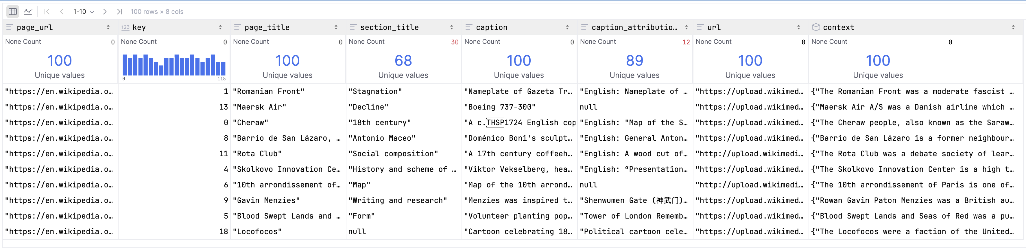
Let’s use Spiral CLI to explore the structure of the table (the output is truncated).


spiral tables manifests --project example --table media-table


Key Space manifest
131 fragments, total: 60.6MB, avg: 473.5KB, metadata: 431.7KB
┏━━━━━━━━━━━━┳━━━━━━━━━━━━━━━━━┳━━━━━━━━┳━━━━━━━━━━━━┳━━━━━━━┳━━━━━━━━━━━━━━━━━━━━━━━━━━━━━━━━━━┳━━━━━━━━━━━━━━┓
┃ ID         ┃ Size (Metadata) ┃ Format ┃  Key Span  ┃ Level ┃           Committed At           ┃ Compacted At ┃
┡━━━━━━━━━━━━╇━━━━━━━━━━━━━━━━━╇━━━━━━━━╇━━━━━━━━━━━━╇━━━━━━━╇━━━━━━━━━━━━━━━━━━━━━━━━━━━━━━━━━━╇━━━━━━━━━━━━━━┩
│ 0qaq87gz87 │ 30.4MB (19.6KB) │ vortex │ 0..1294000 │  L0   │ 2025-11-06 18:20:00.224537+00:00 │     N/A      │


Column Group manifest for table_sl6o0u
6 fragments, total: 113.9MB, avg: 19.0MB, metadata: 111.5KB
┏━━━━━━━━━━━━┳━━━━━━━━━━━━━━━━━┳━━━━━━━━┳━━━━━━━━━━━━━━━━━━┳━━━━━━━┳━━━━━━━━━━━━━━━━━━━━━━━━━━━━━━━━━━┳━━━━━━━━━━━━━━┓
┃ ID         ┃ Size (Metadata) ┃ Format ┃     Key Span     ┃ Level ┃           Committed At           ┃ Compacted At ┃
┡━━━━━━━━━━━━╇━━━━━━━━━━━━━━━━━╇━━━━━━━━╇━━━━━━━━━━━━━━━━━━╇━━━━━━━╇━━━━━━━━━━━━━━━━━━━━━━━━━━━━━━━━━━╇━━━━━━━━━━━━━━┩
│ pqjb420f8r │ 20.2MB (19.1KB) │ vortex │    0..228261     │  L0   │ 2025-11-06 18:20:00.224537+00:00 │     N/A      │
│ vrv19qwg1i │ 20.2MB (19.1KB) │ vortex │  228261..456522  │  L0   │ 2025-11-06 18:20:00.224537+00:00 │     N/A      │
│ 9lhiuacvoi │ 20.0MB (19.1KB) │ vortex │  456522..684783  │  L0   │ 2025-11-06 18:20:00.224537+00:00 │     N/A      │
│ yq7dqeed9r │ 20.1MB (19.1KB) │ vortex │  684783..913044  │  L0   │ 2025-11-06 18:20:00.224537+00:00 │     N/A      │
│ 2tbvh0v6td │ 20.1MB (19.1KB) │ vortex │ 913044..1141305  │  L0   │ 2025-11-06 18:20:00.224537+00:00 │     N/A      │
│ d4xlsgo7ff │ 13.3MB (16.1KB) │ vortex │ 1141305..1294000 │  L0   │ 2025-11-06 18:20:00.224537+00:00 │     N/A      │


Column Group manifest for table_sl6o0u.context
11 fragments, total: 2.6GB, avg: 120.9MB, metadata: 2.7MB
┏━━━━━━━━━━━━┳━━━━━━━━━━━━━━━━━┳━━━━━━━━┳━━━━━━━━━━━━━┳━━━━━━━┳━━━━━━━━━━━━━━━━━━━━━━━━━━━━━━━━━━┳━━━━━━━━━━━━━━┓
┃ ID         ┃ Size (Metadata) ┃ Format ┃  Key Span   ┃ Level ┃           Committed At           ┃ Compacted At ┃
┡━━━━━━━━━━━━╇━━━━━━━━━━━━━━━━━╇━━━━━━━━╇━━━━━━━━━━━━━╇━━━━━━━╇━━━━━━━━━━━━━━━━━━━━━━━━━━━━━━━━━━╇━━━━━━━━━━━━━━┩
│ xn6rq15db4 │ 129.5MB (2.4KB) │ vortex │   0..1177   │  L0   │ 2025-11-06 20:10:41.359348+00:00 │     N/A      │
│ vn4d04pp2r │ 128.7MB (2.4KB) │ vortex │ 1177..2354  │  L0   │ 2025-11-06 20:10:41.359348+00:00 │     N/A      │
│ yqgn69c1rh │ 126.2MB (2.4KB) │ vortex │ 2354..3531  │  L0   │ 2025-11-06 20:10:41.359348+00:00 │     N/A      │
│ 9mmqc78utg │ 129.3MB (2.4KB) │ vortex │ 3531..4708  │  L0   │ 2025-11-06 20:10:41.359348+00:00 │     N/A      │
│ ffsgw7yf5m │ 126.6MB (2.4KB) │ vortex │ 4708..5885  │  L0   │ 2025-11-06 20:10:41.359348+00:00 │     N/A      │
│ 3319x978du │ 127.5MB (2.4KB) │ vortex │ 5885..7062  │  L0   │ 2025-11-06 20:10:41.359348+00:00 │     N/A      │

Enrich with Data

Our metadata table has URLs pointing to images. Let’s use Table Enrichment to fetch the images and store them directly into the table. Using Expressions we can define how to derive new columns (like image) from existing columns (like url).


from spiral import expressions as se
 
enrichment = table.enrich(
    {
        "image": se.http.get(table["url"])
    }
)

There are different ways to run the enrichment, but in this case let’s execute it in a streaming fashion since it is the simplest.


enrichment.apply()

se.http.get fetches the image data from the URL as well as some useful metadata. It creates two columns groups, image (with the raw image bytes in bytes column) and image.meta (with metadata such as status code). Our table now looks like this:


table.schema()


pa.schema({
    "page_url": pa.string_view(),
    "key": pa.int64(),
    "page_title": pa.string_view(),
    "section_title": pa.string_view(),
    "caption": pa.string_view(),
    "caption_attribution_description": pa.string_view(),
    "url": pa.string_view(),
    "context": pa.struct({
        "page_description": pa.string_view(),
        "section_description": pa.string_view()
    }),
    "image": pa.struct({
        "bytes": pa.binary_view(),
        "meta": pa.struct({
            "location": pa.string_view(),
            "last_modified": pa.int64(),
            "size": pa.uint64(),
            "e_tag": pa.string_view(),
            "version": pa.string_view(),
            "status_code": pa.uint16()
        })
    })
})

Let’s use Spiral CLI to explore the updated structure of the table (the output is truncated). We expect to see two new column groups: image and image.meta.


spiral tables manifests --project example --table media-table


Column Group manifest for table_sl6o0u.image
1165 fragments, total: 137.6GB, avg: 120.9MB, metadata: 2.7MB
┏━━━━━━━━━━━━┳━━━━━━━━━━━━━━━━━┳━━━━━━━━┳━━━━━━━━━━━━━┳━━━━━━━┳━━━━━━━━━━━━━━━━━━━━━━━━━━━━━━━━━━┳━━━━━━━━━━━━━━┓
┃ ID         ┃ Size (Metadata) ┃ Format ┃  Key Span   ┃ Level ┃           Committed At           ┃ Compacted At ┃
┡━━━━━━━━━━━━╇━━━━━━━━━━━━━━━━━╇━━━━━━━━╇━━━━━━━━━━━━━╇━━━━━━━╇━━━━━━━━━━━━━━━━━━━━━━━━━━━━━━━━━━╇━━━━━━━━━━━━━━┩
│ xn6rq15db4 │ 129.5MB (2.4KB) │ vortex │   0..1177   │  L0   │ 2025-11-06 20:10:41.359348+00:00 │     N/A      │
│ vn4d04pp2r │ 128.7MB (2.4KB) │ vortex │ 1177..2354  │  L0   │ 2025-11-06 20:10:41.359348+00:00 │     N/A      │
│ yqgn69c1rh │ 126.2MB (2.4KB) │ vortex │ 2354..3531  │  L0   │ 2025-11-06 20:10:41.359348+00:00 │     N/A      │
│ 9mmqc78utg │ 129.3MB (2.4KB) │ vortex │ 3531..4708  │  L0   │ 2025-11-06 20:10:41.359348+00:00 │     N/A      │
│ ffsgw7yf5m │ 126.6MB (2.4KB) │ vortex │ 4708..5885  │  L0   │ 2025-11-06 20:10:41.359348+00:00 │     N/A      │
│ 3319x978du │ 127.5MB (2.4KB) │ vortex │ 5885..7062  │  L0   │ 2025-11-06 20:10:41.359348+00:00 │     N/A      │


Column Group manifest for table_sl6o0u.image.meta
130 fragments, total: 1.5MB, avg: 12.0KB, metadata: 977.8KB
┏━━━━━━━━━━━━┳━━━━━━━━━━━━━━━━━┳━━━━━━━━┳━━━━━━━━━━┳━━━━━━━┳━━━━━━━━━━━━━━━━━━━━━━━━━━━━━━━━━━┳━━━━━━━━━━━━━━┓
┃ ID         ┃ Size (Metadata) ┃ Format ┃ Key Span ┃ Level ┃           Committed At           ┃ Compacted At ┃
┡━━━━━━━━━━━━╇━━━━━━━━━━━━━━━━━╇━━━━━━━━╇━━━━━━━━━━╇━━━━━━━╇━━━━━━━━━━━━━━━━━━━━━━━━━━━━━━━━━━╇━━━━━━━━━━━━━━┩
│ cyjkjdaezp │  11.8KB (7.5KB) │ vortex │ 0..10000 │  L0   │ 2025-11-06 20:10:41.359348+00:00 │     N/A      │
│ cmcb44n6z6 │  12.2KB (7.5KB) │ vortex │ 0..10000 │  L0   │ 2025-11-06 20:10:41.359348+00:00 │     N/A      │
│ t5vovxqks2 │  12.3KB (7.6KB) │ vortex │ 0..10000 │  L0   │ 2025-11-06 20:10:41.359348+00:00 │     N/A      │
│ gof24kc956 │  12.2KB (7.5KB) │ vortex │ 0..10000 │  L0   │ 2025-11-06 20:10:41.359348+00:00 │     N/A      │
│ x6ujppiw06 │  11.8KB (7.5KB) │ vortex │ 0..10000 │  L0   │ 2025-11-06 20:10:41.359348+00:00 │     N/A      │
│ r0gesz2qpe │  12.1KB (7.6KB) │ vortex │ 0..10000 │  L0   │ 2025-11-06 20:10:41.359348+00:00 │     N/A      │

Explore Tables

The entry point for reading data from Spiral Tables is scan and Scan Object.

Let’s explore failures in our enrichment by scanning the table and filtering on image.meta.status_code.


scan = sp.scan(
    table[["url", "image.meta.status_code"]],
    where=table["image.meta.status_code"] != pa.scalar(200, pa.uint16()),
)

Let’s check if the result is what we expect.


scan.schema()


pa.schema({
    "url": pa.string_view(),
    "image": pa.struct({
        "meta": pa.struct({
            "status_code": pa.uint16(),
        }),
    }),
})

Let’s execute the scan and check the results.


scan.to_polars()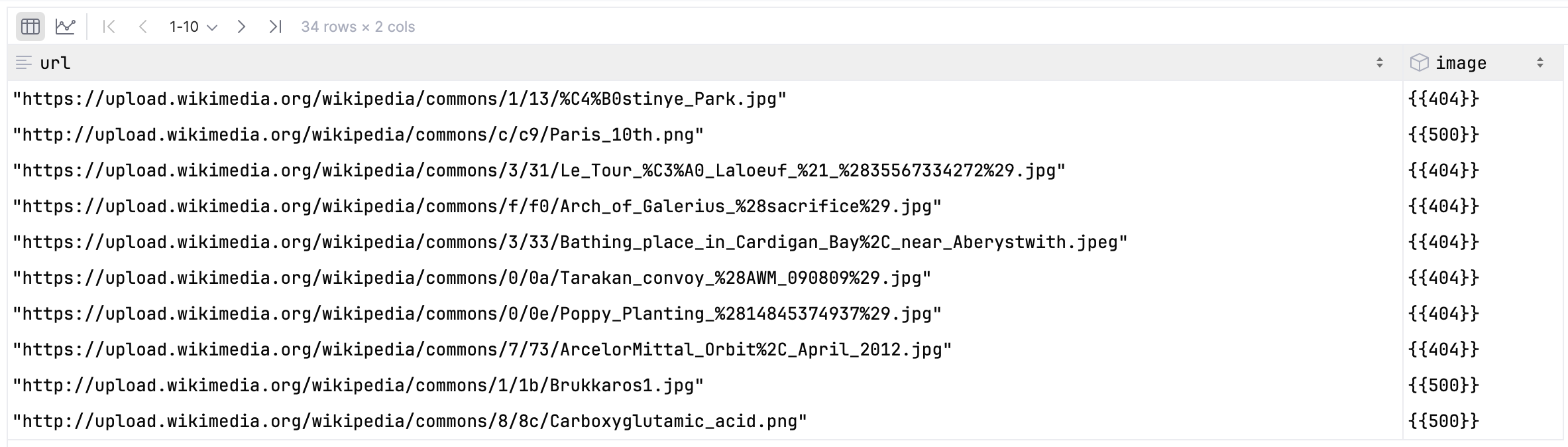

Failed Enrichments

Nice! Only a few failed enrichments, and most of them are 404 Not Found errors as expected.

Now let’s get images from a specific page URL.


sp.scan(
    table["image"][["bytes"]],
    where=(table["page_url"] == "https://en.wikipedia.org/wiki/Ballona_Creek")
).to_table().to_pydict()


{'bytes': [b'\x89PNG\r\n\x1a\n\x00\x00\x00\rIHDR\x00\x00\x03G\x00\x00\x02h\x08\x03\x00\x00\x00\x9a\xe9j\xe6\x00\x00\x03\x00PLTE\xff\xff\xff\xde\xde\xdeBBB::B!1)B:)RRR\x9c\x9c\x94\xce\xce\xc5\xbd\xbd\xd6\xbd\xbd\xbd\x9c\xa5\xb5\xbd\xc5\xc5\xad\xa...

High Throughput Scans

Spiral Tables are designed for high-throughput scans.

Getting a stream of record batches from any scan as simpler as this:


sp.scan(table["image"][["bytes"]]).to_record_batches()

Checkout the API Reference for more details on how to customize scans.

Distributing Work

Many scan functions accepts shards. Shards are row-wise partitions of the table that are defined by exclusive key ranges and can be processed in parallel. Using shards, you can scale out scans to thousands of workers. Shards can be obtained via shards() or built using compute_shards().

Scans represent physical plans and can be sent to remote workers for execution. To get a serializable representation of a scan, use state_json() that can be resumed later, on a different client, via resume_scan().

Data Loading

Getting a PyTorch-compatible data loader from any scan as simple as this:


sp.scan(table["image"][["bytes"]]).to_data_loader(batch_size=32)

SpiralDataLoader supports shard-level shuffling and in-memory shuffling via shuffle buffer.